> #######################################################################
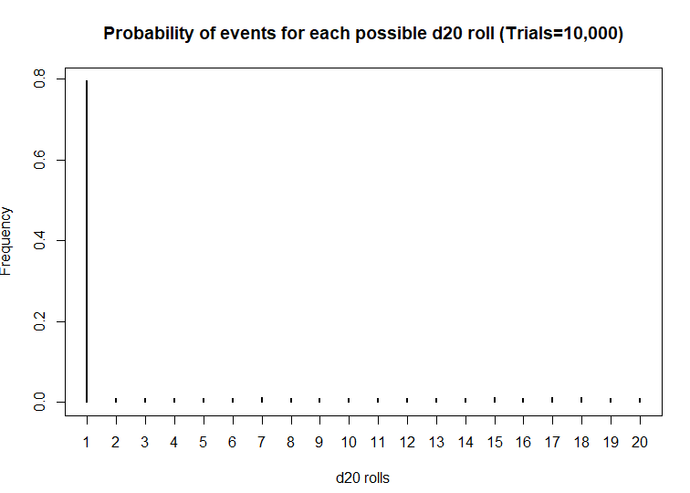
> ## Simulate a d20 dice roll with 10000 trials -- BIASED sample
> ## This is a biased d20 where the number 1 has an 80% probability of hitting.
> #######################################################################
> sims <- sample(x = 1:20, size=10000, prob=c(0.8, 0.01052632, 0.01052632, 0.01052632, 0.01052632, 0.01052632, 0.01052632, 0.01052632, 0.01052632, 0.01052632, 0.01052632, 0.01052632, 0.01052632, 0.01052632, 0.01052632, 0.01052632, 0.01052632, 0.01052632, 0.01052632, 0.01052632), replace=TRUE)
>
> ## Generate frequency table
> table(sims)
sims
1 2 3 4 5 6 7 8 9 10 11 12 13 14 15 16 17 18 19 20
7952 99 104 111 111 104 120 109 98 93 107 99 107 110 116 109 118 122 104 107
>
> ## Generate probability table
> prob <- table(sims) / length(sims)
>
> ## Plot the frequency of the rolls
> plot(table(sims), xlab = 'd20 rolls', ylab = 'Frequency', main = 'Frequency of events for each possible d20 roll (Trials=10,000)')
>
> ## Plot the probability of the rolls
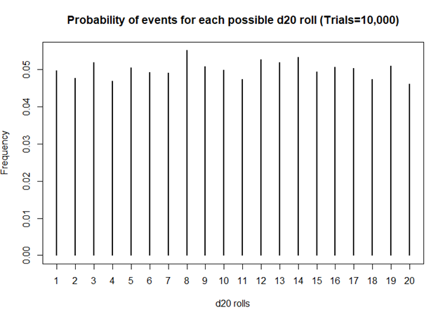
> plot(prob, xlab = 'd20 rolls', ylab = 'Frequency', main = 'Probability of events for each possible d20 roll (Trials=10,000)')
>
> ## Perform chi square test
> chi2 <- chisq.test(table(sims))
> chi2
Chi-squared test for given probabilities
data: table(sims)
X-squared = 116910, df = 19, p-value < 2.2e-16